Module 3 | Lesson 2 | Fly-CURE - Assessing Read Quality

Overview

Teaching: 0 min
Exercises: 0 min

Questions

How can I describe the quality of my data?

Objectives

Explain how a FASTQ file encodes per-base quality scores.

Interpret a FastQC plot summarizing per-base quality across all reads.

Use for loops to automate operations on multiple files.

Run FastQC on fly NGS FASTQ files.

Recorded Lesson:

Bioinformatic workflows

When working with high-throughput sequencing data, the raw reads you get off of the sequencer will need to pass through a number of different tools in order to generate your final desired output. The execution of this set of tools in a specified order is commonly referred to as a workflow or a pipeline.

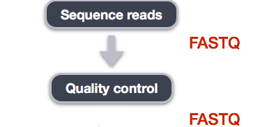
An example of the workflow we will be using for our variant calling analysis is provided below with a brief description of each step.

workflow

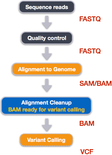
Quality control - Assessing quality using FastQC
Quality control - Trimming and/or filtering reads (if necessary)
Align reads to reference genome
Perform post-alignment clean-up
Variant calling

These workflows in bioinformatics adopt a plug-and-play approach in that the output of one tool can be easily used as input to another tool without any extensive configuration. Having standards for data formats is what makes this feasible. Standards ensure that data is stored in a way that is generally accepted and agreed upon within the community. The tools that are used to analyze data at different stages of the workflow are therefore built under the assumption that the data will be provided in a specific format.

Starting with Data

Often times, the first step in a bioinformatic workflow is getting the data you want to work with onto a computer where you can work with it. If you have outsourced sequencing of your data, the sequencing center will usually provide you with a link that you can use to download your data. We will be using data deposited into an NCBI BioProject (PRJNA779740) which contains all sequenced EMS Drosophila melanogaster genomes to date.

A raw_illumina directory was received directly from the Illumina sequencer. There are 2 files for each mutant Drosophila representing the paired-end reads, R1 (read 1) and R2 (read 2). Each of the .fastq files have been uploaded to a BioSample within the BioProject. To obtain the data, we will use a either a curl or wget command to upload the data to your CyVerse instance.

Launch your app as you always have with the dataset set to: /iplant/home/your_username/data (or use the terminal you currently have opened). (Replace the your_username with your actual username).

We are going to start by downloading data to a local directory which allows the processes to run more quickly without the data saving to your data store within CyVerse. The danger of this is, if you don’t save your data it will be lost when you close your analysis. We will save data as necessary as there is a limit to data storage under the Basic subscription tier.

Here we are using the -p option for mkdir. This option allows mkdir to create the new directory, even if one of the parent directories doesn’t already exist. It also suppresses errors if the directory already exists, without overwriting that directory.

mkdir -p ~/home/your_username/FlyCURE/fastq_joined
cd ~/home/your_username/FlyCURE/fastq_joined

Next, select 5 mutant genomes to download and analyze for this course. This is the link to access all genomes sequenced to date to select from. If you participated in the FlyCURE, you can likely find the mutant your class studied!

After you select your 5 mutants, you will need to upload a total of 10 files using the commands below as an example. You must upload both Read 1 (R1) and Read 2 (R2) for every sample. (The links below will NOT work.) Note: You can run the analysis on ALL of the samples we have sequenced however, that is out of the scope and resources available for this course.

curl -O https://data.cyverse.org/dav-anon/iplant/home/kbieser/FlyCURE_class/fastq_joined/F-1-4_R1.fastq.gz
curl -O https://data.cyverse.org/dav-anon/iplant/home/kbieser/FlyCURE_class/fastq_joined/F-1-4_R2.fastq.gz
curl -O https://data.cyverse.org/dav-anon/iplant/home/kbieser/FlyCURE_class/fastq_joined/G-3-4_R1.fastq.gz
curl -O https://data.cyverse.org/dav-anon/iplant/home/kbieser/FlyCURE_class/fastq_joined/G-3-4_R2.fastq.gz
curl -O https://data.cyverse.org/dav-anon/iplant/home/kbieser/FlyCURE_class/fastq_joined/L-3-2_R1.fastq.gz
curl -O https://data.cyverse.org/dav-anon/iplant/home/kbieser/FlyCURE_class/fastq_joined/L-3-2_R2.fastq.gz
curl -O https://data.cyverse.org/dav-anon/iplant/home/kbieser/FlyCURE_class/fastq_joined/N-1-1_R1.fastq.gz
curl -O https://data.cyverse.org/dav-anon/iplant/home/kbieser/FlyCURE_class/fastq_joined/N-1-1_R2.fastq.gz
curl -O https://data.cyverse.org/dav-anon/iplant/home/kbieser/FlyCURE_class/fastq_joined/O-2-2_R1.fastq.gz
curl -O https://data.cyverse.org/dav-anon/iplant/home/kbieser/FlyCURE_class/fastq_joined/O-2-2_R2.fastq.gz

Verify that the file sizes match those listed in the spreadsheet before proceeding. If they don’t match, try to upload again or reach out to your professor.

$ cd ~/home/your_username/FlyCURE/fastq_joined
$ ls -lh

The file names may be long and have more information than we need. If this is the case for the samples you selected, let’s simplify the file names using a mv command. The mv command in this case, moves the file from its current name into a file with a new, simplified name. The only information we need to keep is the mutant name, in this example M-2-2, the read, R1, and the file suffix, fastq.gz (remove the .1 after the .gz if present). All the other information can be eliminated. If your sample names are already simplified, you can skip this step.

$ cd ~/home/your_username/FlyCURE/fastq_joined
$ mv M-2-2_S4_L001_R1_001.fastq.gz.1 M-2-2_R1.fastq.gz

Continue to rename all of your sequence files in the same fashion before proceeding.

The data in the fastq_joined directory comes in a compressed format, which is why there is a .gz at the end of the file names. This makes it faster to transfer, and allows it to take up less space on our computer. Let’s unzip one of the files so that we can look at the fastq format.

If you recall, we can use the gunzip command to unzip ‘.gz’ files. Since these files are much larger than the data sets we have worked with previously, it may take a few minutes to unzip.

$ cd ~/home/your_username/FlyCURE/fastq_joined
$ gunzip G-3-4_R1.fastq.gz

Quality Control

We will now assess the quality of the sequence reads contained in our fastq files.

workflow_qc

Details on the FASTQ format

Although it looks complicated (and it is), we can understand FASTQ format with a little decoding. Click here for a link to additional information about the FASTQ format. Some rules about the format include…

Line	Description
1	Always begins with ‘@’ and then information about the read
2	The actual DNA sequence
3	Always begins with a ‘+’ and sometimes the same info in line 1
4	Has a string of characters which represent the quality scores; must have same number of characters as line 2

We can view the first complete read in one of the files our dataset by using head to look at the first four lines.

$ head -n 4 G-3-4_R1.fastq

@NB551592:7:HN2MLAFX2:1:11101:19521:1015 1:N:0:TGACCA
NTATTTATAAAAATAAATCCATTCGAATACGGCCATTTTTATATAGCACTCGTAATTCGTATTTCCATTTTTAAAT
+
#AAAAEEEEEEEEEEEEEEEEEEEAEAEEEEEEAEEEEEEEEEAEEEEEEEEEEAEEEEEEEEEEEEEEEAEEEEE

Line 4 shows the quality for each nucleotide in the read. Quality is interpreted as the probability of an incorrect base call (e.g. 1 in 10) or, equivalently, the base call accuracy (e.g. 90%). To make it possible to line up each individual nucleotide with its quality score, the numerical score is converted into a code where each individual character represents the numerical quality score for an individual nucleotide. For example, in the line above, the quality score line is:

#AAAAEEEEEEEEEEEEEEEEEEEAEAEEEEEEAEEEEEEEEEAEEEEEEEEEEAEEEEEEEEEEEEEEEAEEEEE

The numerical value assigned to each of these characters depends on the sequencing platform that generated the reads. The sequencing machine used to generate our data uses the standard Sanger quality PHRED score encoding, using Illumina version 1.8 onwards. Each character is assigned a quality score between 0 and 41 as shown in the chart below.

Quality encoding: !"#$%&'()*+,-./0123456789:;<=>?@ABCDEFGHIJ
                   |         |         |         |         |
Quality score:    01........11........21........31........41                                

Each quality score represents the probability that the corresponding nucleotide call is incorrect. This quality score is logarithmically based, so a quality score of 10 reflects a base call accuracy of 90%, but a quality score of 20 reflects a base call accuracy of 99%. These probability values are the results from the base calling algorithm and depend on how much signal was captured for the base incorporation.

Looking back at our read:

@NB551592:7:HN2MLAFX2:1:11101:19521:1015 1:N:0:TGACCA
NTATTTATAAAAATAAATCCATTCGAATACGGCCATTTTTATATAGCACTCGTAATTCGTATTTCCATTTTTAAAT
+
#AAAAEEEEEEEEEEEEEEEEEEEAEAEEEEEEAEEEEEEEEEAEEEEEEEEEEAEEEEEEEEEEEEEEEAEEEEE

we can now see that there is a small range of quality scores.

Exercise

What is the last read in the G-3-4_R1.fastq file? How confident are you in this read?
Solution
$ tail -n 4 G-3-4_R1.fastq
@NB551592:7:HN2MLAFX2:4:21612:18302:20422 1:N:0:TGACCA
NTCGGCTAACTGCAATCCTTGAATCCACTGAGAAGTTGCGTCTCCGAGAAACAAATGAGCTGTAAGCTGCGCTGTG
+
#AAAAEEEEEEEEEEEEEEEEEEEEEEEEEEEAEEEEEEEEEEEEEEEEEEEEEEEEAEEEEEEAEEEEEEEEEEA
This read has the same consistent quality at the beginning as compared to the first read that we looked at, but has a wider range of quality scores, with scores becoming lower at the middle to end of the read. We will look at variations in position-based quality in just a moment.

We unzipped one of our files so before we work with it again, let’s compress it.

First, you have to install pigz which will perform zipping faster than gzip which we have previously used.

$ sudo apt-get install pigz

Then, run pigz. This will take a few minutes to run.

$ pigz G-3-4_R1.fastq

At this point, lets validate that all the relevant tools are installed. If you are using JupyterLab then these should be preinstalled.

$ fastqc -h
            FastQC - A high throughput sequence QC analysis tool

SYNOPSIS

        fastqc seqfile1 seqfile2 .. seqfileN

    fastqc [-o output dir] [--(no)extract] [-f fastq|bam|sam]
           [-c contaminant file] seqfile1 .. seqfileN

DESCRIPTION

    FastQC reads a set of sequence files and produces from each one a quality
    control report consisting of a number of different modules, each one of
    which will help to identify a different potential type of problem in your
    data.

    If no files to process are specified on the command line then the program
    will start as an interactive graphical application.  If files are provided
    on the command line then the program will run with no user interaction
    required.  In this mode it is suitable for inclusion into a standardised
    analysis pipeline.

    The options for the program as as follows:

    -h --help       Print this help file and exit

    -v --version    Print the version of the program and exit

    -o --outdir     Create all output files in the specified output directory.                                                                                    
                    Please note that this directory must exist as the program
                    will not create it.  If this option is not set then the
                    output file for each sequence file is created in the same
                    directory as the sequence file which was processed.

    --casava        Files come from raw casava output. Files in the same sample
                    group (differing only by the group number) will be analysed
                    as a set rather than individually. Sequences with the filter
                    flag set in the header will be excluded from the analysis.
                    Files must have the same names given to them by casava
                    (including being gzipped and ending with .gz) otherwise they
                    won't be grouped together correctly.

    --nano          Files come from naopore sequences and are in fast5 format. In
                    this mode you can pass in directories to process and the program
                    will take in all fast5 files within those directories and produce
                    a single output file from the sequences found in all files.

    --nofilter      If running with --casava then don't remove read flagged by
                    casava as poor quality when performing the QC analysis.

    --extract       If set then the zipped output file will be uncompressed in
                    the same directory after it has been created.  By default
                    this option will be set if fastqc is run in non-interactive
                    mode.

    -j --java       Provides the full path to the java binary you want to use to
                    launch fastqc. If not supplied then java is assumed to be in
                    your path.

    --noextract     Do not uncompress the output file after creating it.  You
                    should set this option if you do not wish to uncompress
                    the output when running in non-interactive mode.

    --nogroup       Disable grouping of bases for reads >50bp. All reports will
                    show data for every base in the read.  WARNING: Using this
                    option will cause fastqc to crash and burn if you use it on
                    really long reads, and your plots may end up a ridiculous size.
                    You have been warned!

    -f --format     Bypasses the normal sequence file format detection and
                    forces the program to use the specified format.  Valid
                    formats are bam,sam,bam_mapped,sam_mapped and fastq

    -t --threads    Specifies the number of files which can be processed
                    simultaneously.  Each thread will be allocated 250MB of
                    memory so you shouldn't run more threads than your
                    available memory will cope with, and not more than
                    6 threads on a 32 bit machine

    -c              Specifies a non-default file which contains the list of
    --contaminants  contaminants to screen overrepresented sequences against.
                    The file must contain sets of named contaminants in the
                    form name[tab]sequence.  Lines prefixed with a hash will
                    be ignored.

    -a              Specifies a non-default file which contains the list of
    --adapters      adapter sequences which will be explicity searched against
                    the library. The file must contain sets of named adapters
                    in the form name[tab]sequence.  Lines prefixed with a hash
                    will be ignored.

    -l              Specifies a non-default file which contains a set of criteria
    --limits        which will be used to determine the warn/error limits for the
                    various modules.  This file can also be used to selectively
                    remove some modules from the output all together.  The format
                    needs to mirror the default limits.txt file found in the
                    Configuration folder.

   -k --kmers       Specifies the length of Kmer to look for in the Kmer content
                    module. Specified Kmer length must be between 2 and 10. Default
                    length is 7 if not specified.

   -q --quiet       Supress all progress messages on stdout and only report errors.

   -d --dir         Selects a directory to be used for temporary files written when
                    generating report images. Defaults to system temp directory if
                    not specified.

BUGS

    Any bugs in fastqc should be reported either to simon.andrews@babraham.ac.uk
    or in www.bioinformatics.babraham.ac.uk/bugzilla/

Assessing Quality using FastQC

In real life, you won’t be assessing the quality of your reads by visually inspecting your FASTQ files. Rather, you’ll be using a software program to assess read quality and filter out poor quality reads. We’ll first use a program called FastQC to visualize the quality of our reads. Click this link to take you to FastQC. Later in our workflow, we’ll use another program to filter out poor quality reads.

FastQC has a number of features which can give you a quick impression of any problems your data may have, so you can take these issues into consideration before moving forward with your analyses. Rather than looking at quality scores for each individual read, FastQC looks at quality collectively across all reads within a sample. The image below shows one FastQC-generated plot that indicates a very high quality sample:

good_quality

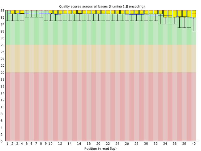
The x-axis displays the base position in the read, and the y-axis shows quality scores. In this example, the sample contains reads that are 40 bp long. This is much shorter than the reads we are working with in our workflow. For each position, there is a box-and-whisker plot showing the distribution of quality scores for all reads at that position. The horizontal red line indicates the median quality score and the yellow box shows the 1st to 3rd quartile range. This means that 50% of reads have a quality score that falls within the range of the yellow box at that position. The whiskers show the absolute range, which covers the lowest (0th quartile) to highest (4th quartile) values.

For each position in this sample, the quality values do not drop much lower than 32. This is a high quality score. The plot background is also color-coded to identify good (green), acceptable (yellow), and bad (red) quality scores.

Now let’s take a look at a quality plot on the other end of the spectrum.

bad_quality

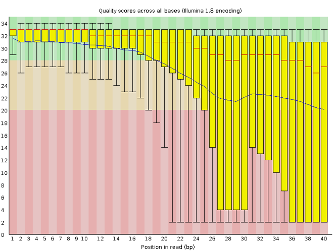
Here, we see positions within the read in which the boxes span a much wider range. Also, quality scores drop quite low into the “bad” range, particularly on the tail end of the reads. The FastQC tool produces several other diagnostic plots to assess sample quality, in addition to the one plotted above.

Running FastQC individual method (script method below - your choice)

We will now assess the quality of the reads that you downloaded. First, make sure you’re still in the local fastq_joined directory.

$ cd ~/home/your_username/FlyCURE/fastq_joined

Exercise

How big are the files? (Hint: Look at the options for the ls command to see how to show file sizes.)

Solution

$ ls -lh

rw-r--r-- 1 gea_user gea_user 3.9G Mar 22 19:26 A44_R1.fastq
-rw-r--r-- 1 gea_user gea_user 956M Mar 22 19:26 A44_R2.fastq.gz
-rw-r--r-- 1 gea_user gea_user 1.3G Mar 22 19:22 B-1-3_R1_001.fastq.gz
-rw-r--r-- 1 gea_user gea_user 1.4G Mar 22 19:22 B-1-3_R2_001.fastq.gz
-rw-r--r-- 1 gea_user gea_user 1.3G Mar 22 19:26 B-2-13_R1.fastq.gz
-rw-r--r-- 1 gea_user gea_user 1.4G Mar 22 19:26 B-2-13_R2.fastq.gz
-rw-r--r-- 1 gea_user gea_user 1.3G Mar 22 19:27 B-2-16_R1.fastq.gz
-rw-r--r-- 1 gea_user gea_user 1.3G Mar 22 19:27 B-2-16_R2.fastq.gz
-rw-r--r-- 1 gea_user gea_user 1.3G Mar 22 19:28 Control_R1.fastq.gz
-rw-r--r-- 1 gea_user gea_user 1.3G Mar 22 19:28 Control_R2.fastq.gz
-rw-r--r-- 1 gea_user gea_user 1.6G Mar 22 19:33 F-1-4_R1.fastq.gz
-rw-r--r-- 1 gea_user gea_user 1.6G Mar 22 19:33 F-1-4_R2.fastq.gz
-rw-r--r-- 1 gea_user gea_user 1.2G Mar 22 19:23 E-2-2_R1_001.fastq.gz
-rw-r--r-- 1 gea_user gea_user 1.2G Mar 22 19:23 E-2-2_R2_001.fastq.gz
-rw-r--r-- 1 gea_user gea_user 1.3G Mar 22 19:24 G-3-4_R1.fastq.gz
-rw-r--r-- 1 gea_user gea_user 1.3G Mar 22 19:24 G-3-4_R2.fastq.gz
-rw-r--r-- 1 gea_user gea_user 1.7G Mar 22 19:28 H22_R1.fastq.gz
-rw-r--r-- 1 gea_user gea_user 1.8G Mar 22 19:29 H22_R2.fastq.gz
-rw-r--r-- 1 gea_user gea_user 1.3G Mar 22 19:24 H-3-2_R1.fastq.gz
-rw-r--r-- 1 gea_user gea_user 1.3G Mar 22 19:25 H-3-2_R2.fastq.gz
-rw-r--r-- 1 gea_user gea_user 1.7G Mar 22 19:30 L31_R1.fastq.gz
-rw-r--r-- 1 gea_user gea_user 1.7G Mar 22 19:31 L31_R2.fastq.gz
-rw-r--r-- 1 gea_user gea_user 1.4G Mar 22 19:29 L-3-2_R1.fastq.gz
-rw-r--r-- 1 gea_user gea_user 1.4G Mar 22 19:30 L-3-2_R2.fastq.gz
-rw-r--r-- 1 gea_user gea_user 1.4G Mar 22 19:31 N-1-1_R1.fastq.gz
-rw-r--r-- 1 gea_user gea_user 1.4G Mar 22 19:31 N-1-1_R2.fastq.gz
-rw-r--r-- 1 gea_user gea_user 1.4G Mar 22 19:32 N-1-4_R1.fastq.gz
-rw-r--r-- 1 gea_user gea_user 1.5G Mar 22 19:32 N-1-4_R2.fastq.gz
-rw-r--r-- 1 gea_user gea_user 1.3G Mar 22 19:25 O-2-2_R1.fastq.gz
-rw-r--r-- 1 gea_user gea_user 1.3G Mar 22 19:25 O-2-2_R2.fastq.gz

You will only see the files for the mutants you are analyzing. Pay attention to the size of the files. They should ranging from 1.2G (1.2 gigabytes) to 1.7G for zipped files. Depending on when the particular sequences you are using were sequenced, file sizes may be larger than these.

FastQC can accept multiple file names as input, and on both zipped and unzipped files, so we can use the .fastq wildcard to run FastQC on all of the FASTQ files in this directory.

$ fastqc *.fastq*

You will see an automatically updating output message telling you the progress of the analysis. It will start like this:

Started analysis of B-2-13_R1.fastq
Approx 5% complete for B-2-13_R1.fastq
Approx 10% complete for B-2-13_R1.fastq

In total, this will take some time for FastQC to run on all five of our FASTQ files. When the analysis completes, your prompt will return. So your screen will look something like this:

Approx 70% complete for N-1-4_R2.fastq.gz
Approx 75% complete for N-1-4_R2.fastq.gz
Approx 80% complete for N-1-4_R2.fastq.gz
Approx 85% complete for N-1-4_R2.fastq.gz
Approx 90% complete for N-1-4_R2.fastq.gz
Approx 95% complete for N-1-4_R2.fastq.gz
Analysis complete for N-1-4_R2.fastq.gz
kbieser@aed3605cf.cyverse.run$

The FastQC program has created several new files within our ~/home/your_username/FlyCURE/fastq_joined directory. (The output will vary based upon the specific mutant samples you are analyzing.)

$ ls -lh

B-2-13_R1.fastq        B-2-13_R2_fastqc.zip   B-2-16_R1.fastq.gz     L-3-2_R1_fastqc.html  L-3-2_R2_fastqc.zip   N-1-1_R1.fastq.gz     
N-1-4_R1_fastqc.html  N-1-4_R2_fastqc.zip     B-2-13_R1_fastqc.html  B-2-13_R2.fastq.gz     B-2-16_R2_fastqc.html  L-3-2_R1_fastqc.zip   
L-3-2_R2.fastq.gz     N-1-1_R2_fastqc.html  N-1-4_R1_fastqc.zip   N-1-4_R2.fastq.gz       B-2-13_R1_fastqc.zip   B-2-16_R1_fastqc.html  
B-2-16_R2_fastqc.zip   L-3-2_R1.fastq.gz     N-1-1_R1_fastqc.html  N-1-1_R2_fastqc.zip   N-1-4_R1.fastq.gz     B-2-13_R2_fastqc.html  
B-2-16_R1_fastqc.zip   B-2-16_R2.fastq.gz     L-3-2_R2_fastqc.html  N-1-1_R1_fastqc.zip   N-1-1_R2.fastq.gz     N-1-4_R2_fastqc.html

For each input FASTQ file, FastQC has created a .zip file and a .html file. The .zip file extension indicates that this is actually a compressed set of multiple output files. We’ll be working with these output files soon. The .html file is a stable webpage displaying the summary report for each of our samples.

We want to keep our data files and our results files separate, so we will move these output files into a new directory within our results/ directory.

*These commands are using an absolute path, but if you are comfortable and understand your file structure feel free to use relative path!

$ mkdir -p ~/home/your_username/FlyCURE/results/fastqc_untrimmed_reads
$ mv *.zip ~/home/your_username/FlyCURE/results/fastqc_untrimmed_reads/
$ mv *.html ~/home/your_username/FlyCURE/results/fastqc_untrimmed_reads/

Now we can navigate into this results directory and do some closer inspection of our output files.

$ cd ~/home/your_username/FlyCURE/results/fastqc_untrimmed_reads/

Running FastQC script method

If you want to run FastQC on all of your files at once and move the outputs to the correct directory, you can write a script to do so.

Let’s start with making a scripts directory to save all the scripts we will be making

$ cd ~/home/your_username/FlyCURE
$ mkdir scripts

Move into the scripts directory

$ cd scripts

$ nano fastqc.sh

In nano type in each command that you want to complete. Let’s also make some notes for ourselves so that we know what to use this script for and where to run it from.

#!/bin/bash
# Use this script to run fastqc on my raw untrimmed reads
# Run me inside of the fastq_trimmed reads directory

mkdir -p ~/home/your_username/FlyCURE/results/fastqc_untrimmed_reads

fastqc -t 10 -o ../results/fastqc_untrimmed_reads *.fastq*

In the FastQC command, the -t 8tells the server how many CPU’s to utilize while running the command. The -o ../results/fastqc_untrimmed_reads, directs where the outputs from fastqc should be saved. In the past we have used the mv command after we ran fastqc, but this method allows the data to be placed in the correct directory upon creation rather than having to move them after the fact. It can do this because we prompted it to make the new directory first ensuring it exists.

Save the script.

To run the script you must make it executable.

$ chmod +x fastqc.sh

Now run the script! Navigate to the correct directory where the script should be run and then call the script.

$ cd ~/home/your_username/FlyCURE/fastq_joined
$ ../scripts/fastqc.sh &

The & will let you follow the progress. This will take some time to complete depending upon how many sequences you are analyzing (plan at least 30 minutes). Remember these are the sequencing reads for the whole genome of Drosophila melanogaster which is approximately 139.5 million base pairs.

Once completed, navigate into the results directory and do some closer inspection of our output files. If any of them failed, run the script again or run fastqc on using the individual sample method above. Those two methods resolved any issues I experienced.

$ cd ~/home/your_username/FlyCURE/results/fastqc_untrimmed_reads

View the files to make sure you have the same file sizes for your samples. It is good practice to continually check your file sizes as they can indicate if your script completed or if there are issues from one step in the analysis to another. I’ve included the output for many of the mutants but not all of them, but this gives you a general idea of file sizes even if your samples are not listed.

$ ls -lh

-rw-r--r-- 1 gea_user gea_user 632K Feb 24 21:10 A44_R1_fastqc.html
-rw-r--r-- 1 gea_user gea_user 435K Feb 24 21:10 A44_R1_fastqc.zip
-rw-r--r-- 1 gea_user gea_user 629K Feb 24 21:10 A44_R2_fastqc.html
-rw-r--r-- 1 gea_user gea_user 432K Feb 24 21:10 A44_R2_fastqc.zip
-rw-r--r-- 1 gea_user gea_user 569K Feb 24 21:11 B-1-3_R1_fastqc.html
-rw-r--r-- 1 gea_user gea_user 390K Feb 24 21:11 B-1-3_R1_fastqc.zip
-rw-r--r-- 1 gea_user gea_user 579K Feb 24 21:11 B-1-3_R2_fastqc.html
-rw-r--r-- 1 gea_user gea_user 394K Feb 24 21:11 B-1-3_R2_fastqc.zip
-rw-r--r-- 1 gea_user gea_user 624K Feb 24 21:11 B-2-13_R1_fastqc.html
-rw-r--r-- 1 gea_user gea_user 404K Feb 24 21:11 B-2-13_R1_fastqc.zip
-rw-r--r-- 1 gea_user gea_user 624K Feb 24 21:11 B-2-13_R2_fastqc.html
-rw-r--r-- 1 gea_user gea_user 408K Feb 24 21:11 B-2-13_R2_fastqc.zip
-rw-r--r-- 1 gea_user gea_user 624K Feb 24 21:11 B-2-16_R1_fastqc.html
-rw-r--r-- 1 gea_user gea_user 401K Feb 24 21:11 B-2-16_R1_fastqc.zip
-rw-r--r-- 1 gea_user gea_user 630K Feb 24 21:11 B-2-16_R2_fastqc.html
-rw-r--r-- 1 gea_user gea_user 412K Feb 24 21:11 B-2-16_R2_fastqc.zip
-rw-r--r-- 1 gea_user gea_user 631K Feb 24 21:11 Control_R1_fastqc.html
-rw-r--r-- 1 gea_user gea_user 432K Feb 24 21:11 Control_R1_fastqc.zip
-rw-r--r-- 1 gea_user gea_user 623K Feb 24 21:11 Control_R2_fastqc.html
-rw-r--r-- 1 gea_user gea_user 424K Feb 24 21:11 Control_R2_fastqc.zip
-rw-r--r-- 1 gea_user gea_user 624K Feb 24 21:11 F-1-4_R1_fastqc.html
-rw-r--r-- 1 gea_user gea_user 418K Feb 24 21:11 F-1-4_R1_fastqc.zip
-rw-r--r-- 1 gea_user gea_user 626K Feb 24 21:11 F-1-4_R2_fastqc.html
-rw-r--r-- 1 gea_user gea_user 425K Feb 24 21:11 F-1-4_R2_fastqc.zip
-rw-r--r-- 1 gea_user gea_user 569K Feb 24 21:11 E-2-2_R1_fastqc.html
-rw-r--r-- 1 gea_user gea_user 390K Feb 24 21:11 E-2-2_R1_fastqc.zip
-rw-r--r-- 1 gea_user gea_user 582K Feb 24 21:11 E-2-2_R2_fastqc.html
-rw-r--r-- 1 gea_user gea_user 395K Feb 24 21:11 E-2-2_R2_fastqc.zip
-rw-r--r-- 1 gea_user gea_user 569K Feb 24 21:11 G-3-4_R1_fastqc.html
-rw-r--r-- 1 gea_user gea_user 391K Feb 24 21:11 G-3-4_R1_fastqc.zip
-rw-r--r-- 1 gea_user gea_user 582K Feb 24 21:11 G-3-4_R2_fastqc.html
-rw-r--r-- 1 gea_user gea_user 396K Feb 24 21:11 G-3-4_R2_fastqc.zip
-rw-r--r-- 1 gea_user gea_user 625K Feb 24 21:11 H22_R1_fastqc.html
-rw-r--r-- 1 gea_user gea_user 420K Feb 24 21:11 H22_R1_fastqc.zip
-rw-r--r-- 1 gea_user gea_user 619K Feb 24 21:11 H22_R2_fastqc.html
-rw-r--r-- 1 gea_user gea_user 414K Feb 24 21:11 H22_R2_fastqc.zip
-rw-r--r-- 1 gea_user gea_user 565K Feb 24 21:11 H-3-2_R1_fastqc.html
-rw-r--r-- 1 gea_user gea_user 387K Feb 24 21:11 H-3-2_R1_fastqc.zip
-rw-r--r-- 1 gea_user gea_user 578K Feb 24 21:11 H-3-2_R2_fastqc.html
-rw-r--r-- 1 gea_user gea_user 392K Feb 24 21:11 H-3-2_R2_fastqc.zip
-rw-r--r-- 1 gea_user gea_user 624K Feb 24 21:11 L31_R1_fastqc.html
-rw-r--r-- 1 gea_user gea_user 415K Feb 24 21:11 L31_R1_fastqc.zip
-rw-r--r-- 1 gea_user gea_user 620K Feb 24 21:11 L31_R2_fastqc.html
-rw-r--r-- 1 gea_user gea_user 415K Feb 24 21:11 L31_R2_fastqc.zip
-rw-r--r-- 1 gea_user gea_user 623K Feb 24 21:11 L-3-2_R1_fastqc.html
-rw-r--r-- 1 gea_user gea_user 399K Feb 24 21:11 L-3-2_R1_fastqc.zip
-rw-r--r-- 1 gea_user gea_user 630K Feb 24 21:11 L-3-2_R2_fastqc.html
-rw-r--r-- 1 gea_user gea_user 411K Feb 24 21:11 L-3-2_R2_fastqc.zip
-rw-r--r-- 1 gea_user gea_user 626K Feb 24 21:11 N-1-1_R1_fastqc.html
-rw-r--r-- 1 gea_user gea_user 405K Feb 24 21:11 N-1-1_R1_fastqc.zip
-rw-r--r-- 1 gea_user gea_user 630K Feb 24 21:11 N-1-1_R2_fastqc.html
-rw-r--r-- 1 gea_user gea_user 415K Feb 24 21:11 N-1-1_R2_fastqc.zip
-rw-r--r-- 1 gea_user gea_user 623K Feb 24 21:11 N-1-4_R1_fastqc.html
-rw-r--r-- 1 gea_user gea_user 402K Feb 24 21:11 N-1-4_R1_fastqc.zip
-rw-r--r-- 1 gea_user gea_user 623K Feb 24 21:11 N-1-4_R2_fastqc.html
-rw-r--r-- 1 gea_user gea_user 410K Feb 24 21:11 N-1-4_R2_fastqc.zip
-rw-r--r-- 1 gea_user gea_user 573K Feb 24 21:11 O-2-2_R1_fastqc.html
-rw-r--r-- 1 gea_user gea_user 392K Feb 24 21:11 O-2-2_R1_fastqc.zip
-rw-r--r-- 1 gea_user gea_user 580K Feb 24 21:11 O-2-2_R2_fastqc.html
-rw-r--r-- 1 gea_user gea_user 394K Feb 24 21:11 O-2-2_R2_fastqc.zip

Viewing the FastQC results

If we were working on our local computers, we’d be able to look at each of these HTML files by opening them in a web browser.

However, these files are currently sitting on our remote CyVerse instance, where our local computer can’t see them.

The traditional way to look at these webpage summary reports would be to transfer them to our local computers (i.e. your laptop). Since we are utilizing the JupyterLab app, we can just navigate to the directory and view them directly in JupyterLab.

In the left hand side of your console, navigate to the .html files.

home/your_username/FlyCURE/results/fastqc_untrimmed_reads

G-3-4_R1.fastqc.html

Double-click on one of the .html files and a new tab will automatically open with the FastQC Report. Open and review each of the fastqc.html files. View the next section for information about decoding the FastQC outputs. Be sure to add your analysis to your notebook.

Exercise

View each of the FastQC reports. Which sample(s) looks the best in terms of per base sequence quality? Which sample(s) look the worst? Write some notes about what you are seeing in your notebook.

Solution

Since we conducted paired-end sequencing, there are two reads for each fastq. A R1 (read 1) and a R2 (read 2). Each sequencing file has usable data, but the quality decreases » toward the end of the reads. R2 has poorer quality than R1.

Decoding the other FastQC outputs

We’ve now looked at quite a few “Per base sequence quality” FastQC graphs, but there are nine other graphs that we haven’t talked about! Below we have provided a brief overview of interpretations for each of these plots. For more information, please see the FastQC documentation by clicking this link

Per tile sequence quality: the machines that perform sequencing are divided into tiles. This plot displays patterns in base quality along these tiles. Consistently low scores are often found around the edges, but hot spots can also occur in the middle if an air bubble was introduced at some point during the run.
Per sequence quality scores: a density plot of quality for all reads at all positions. This plot shows what quality scores are most common.
Per base sequence content: plots the proportion of each base position over all of the reads. Typically, we expect to see each base roughly 25% of the time at each position, but this often fails at the beginning or end of the read due to quality or adapter content.
Per sequence GC content: a density plot of average GC content in each of the reads.
Per base N content: the percent of times that ‘N’ occurs at a position in all reads. If there is an increase at a particular position, this might indicate that something went wrong during sequencing.
Sequence Length Distribution: the distribution of sequence lengths of all reads in the file. If the data is raw, there is often on sharp peak, however if the reads have been trimmed, there may be a distribution of shorter lengths.
Sequence Duplication Levels: A distribution of duplicated sequences. In sequencing, we expect most reads to only occur once. If some sequences are occurring more than once, it might indicate enrichment bias (e.g. from PCR). If the samples are high coverage (or RNA-seq or amplicon), this might not be true.
Overrepresented sequences: A list of sequences that occur more frequently than would be expected by chance.
Adapter Content: a graph indicating where adapater sequences occur in the reads.
K-mer Content: a graph showing any sequences which may show a positional bias within the reads.

Key Points

for loops let you perform the same set of operations on multiple files with a single command.

FastQC enables us to validate the continued use of the sequencing data.

previous episode

Fly-CURE: Shell Genomics, Data Wrangling, and SNP Analyses

next episode

Module 3 | Lesson 2 | Fly-CURE - Assessing Read Quality

Overview

Recorded Lesson:

Bioinformatic workflows

Starting with Data

Quality Control

Details on the FASTQ format

Exercise

Solution

Assessing Quality using FastQC

Running FastQC individual method (script method below - your choice)

Exercise

Solution

Running FastQC script method

Viewing the FastQC results

Exercise

Solution

Decoding the other FastQC outputs

Key Points

previous episode

next episode