Overview

Teaching: 0 min
Exercises: 0 min

Questions

• Can you identify the SNP causing the mutant phenotype?

• What changes would you make to the bioinformatics pipeline?

• What additional experiments would you conduct to verify the presumptive mutant SNP?

Objectives

• Use RStudio to generate list of unique SNPs for each mutant fly stock.

Recorded Lesson:

Module 3 | Lesson 8 | Fly-CURE - Final Identification of SNPs

Required Software

Download Pulsar Text Editor: Link to Pulsar Download Scroll down to “Regular Releases” and choose your operating system for installation and follow the directions for the installer.

Download R: Link to download R Select the download for your operating system and install.

Download Rstudio: Link to download Rstudio Follow step 2 and install Rstudio. If you scroll down, there is a download for both Mac and Windows.

Downloading files from CyVerse to local machine

The final output of SnpEff and SnpSift generates a number of files. The file we need for our last analysis is the *.uniqID.txt for each of the fly stocks you are analyzing.

• Step 1: Create a folder on your personal computer. (i.e. in Documents, Dropbox, Desktop)
• Step 2: Download all of the *.uniqID.txt files located in the /snpeff_bdgp6.86 directory in the Discovery Environment Data Store and save them to the folder on your computer (Fig. 1).

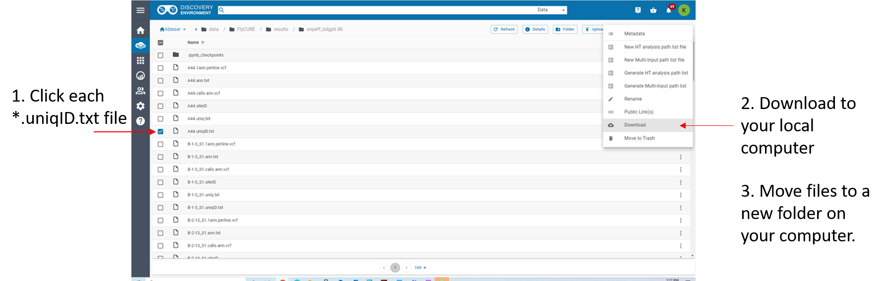Figure 1: Steps to move files to local machine from CyVerse Discovery Environment.

Edit text files

The text files still contain more information than we need, but before we can finalize our data analysis we will need to modify the headers in the text files first. We will use the text editor, Pulsar, to edit the headers. When SnpSift was run, the script sorted the data into 11 columns each containing a column header. You can view these column headers in each of the text files or view them in CyVerse.

$ cd ~/FlyCURE/results/snpeff_bdgp6.86
$ head -n 1 A44.uniqID.txt

CHROM_POS_REF_ANN[*].ALLELE_ANN[*].GENEID_ANN[*].EFFECT CHROM   POS     REF     ANN[*].ALLELE   ANN[*].GENEID   ANN[*].EFFECT   ANN[*].HGVS_P   AF1     ANN[*].IMPACT   ANN[*].GENE

As you can see, the column headers contain no sample specific identifying information and some of them are long. You should see the same 11 columns for each of the fly stocks you are analyzing. The first step for the analysis will require us to edit the column headers so that each is identifiable by our sample/fly stock. There are a few different approaches you can utilize to edit the header. I demonstrate this in a Microsoft Stream video and in the following set of figures. The header for each sample should be identical to the output below with the respective sample name substituted. Do not add spaces or periods in any of the sample names. (i.e. B.2.16 would be entered as B216). The spacing and editing has to be exact or the Rscript will not work!

site_eff_uniq_string	A44_CHROM	A44_POS	A44_REF	A44_ALLELE	A44_GENEID	A44_EFFECT	A44_HGVS_P	A44_AF1	A44_IMPACT	A44_GENE

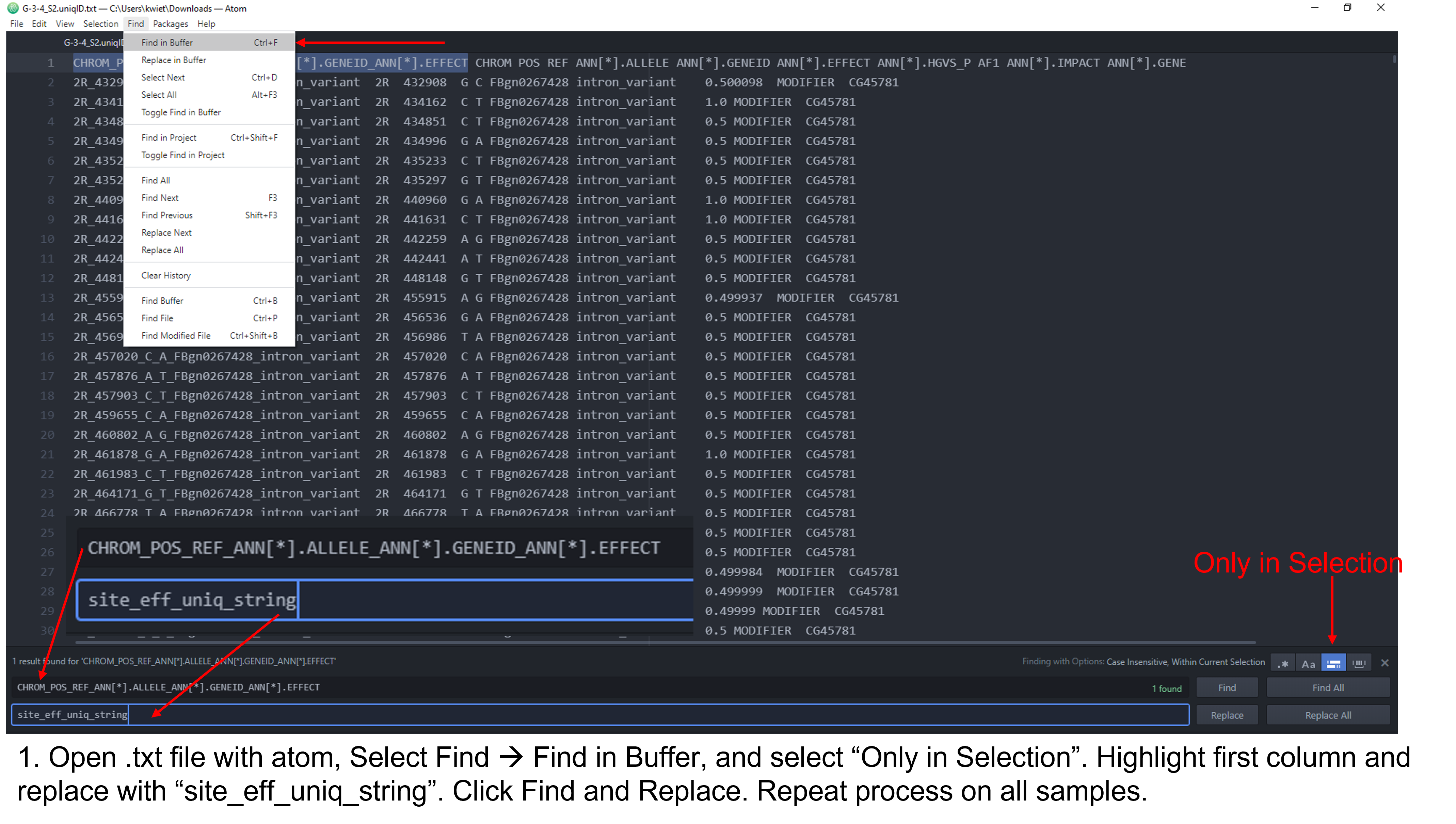
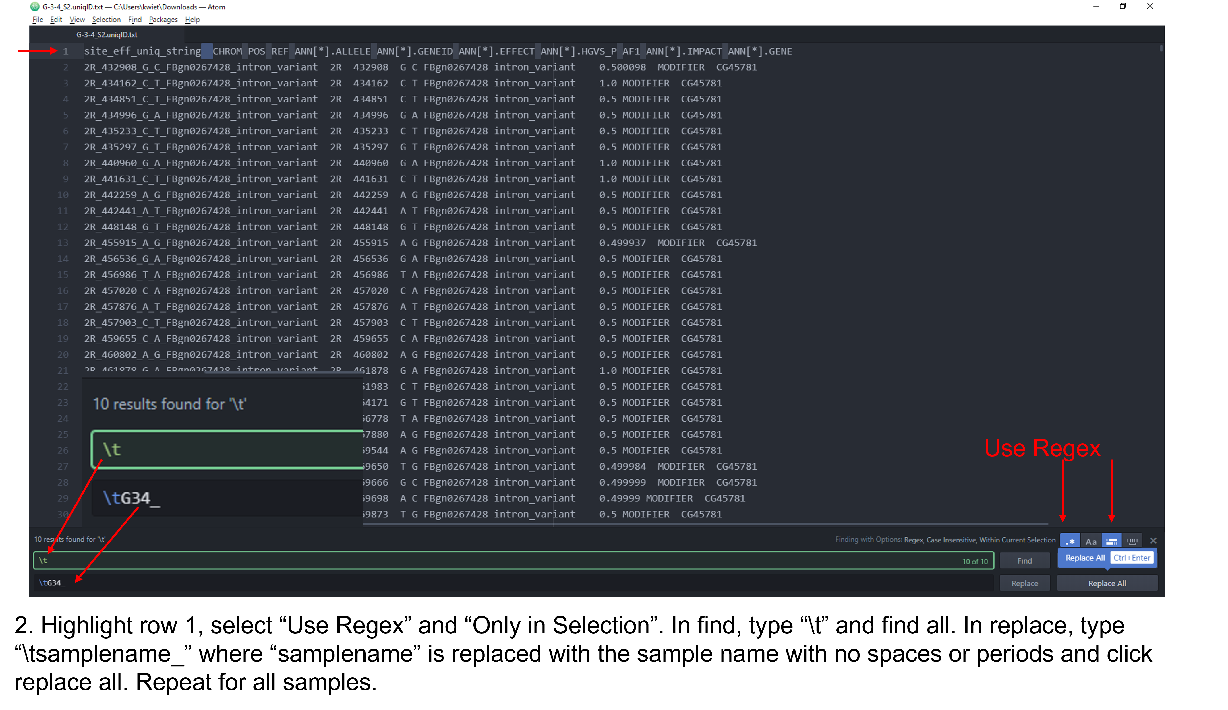
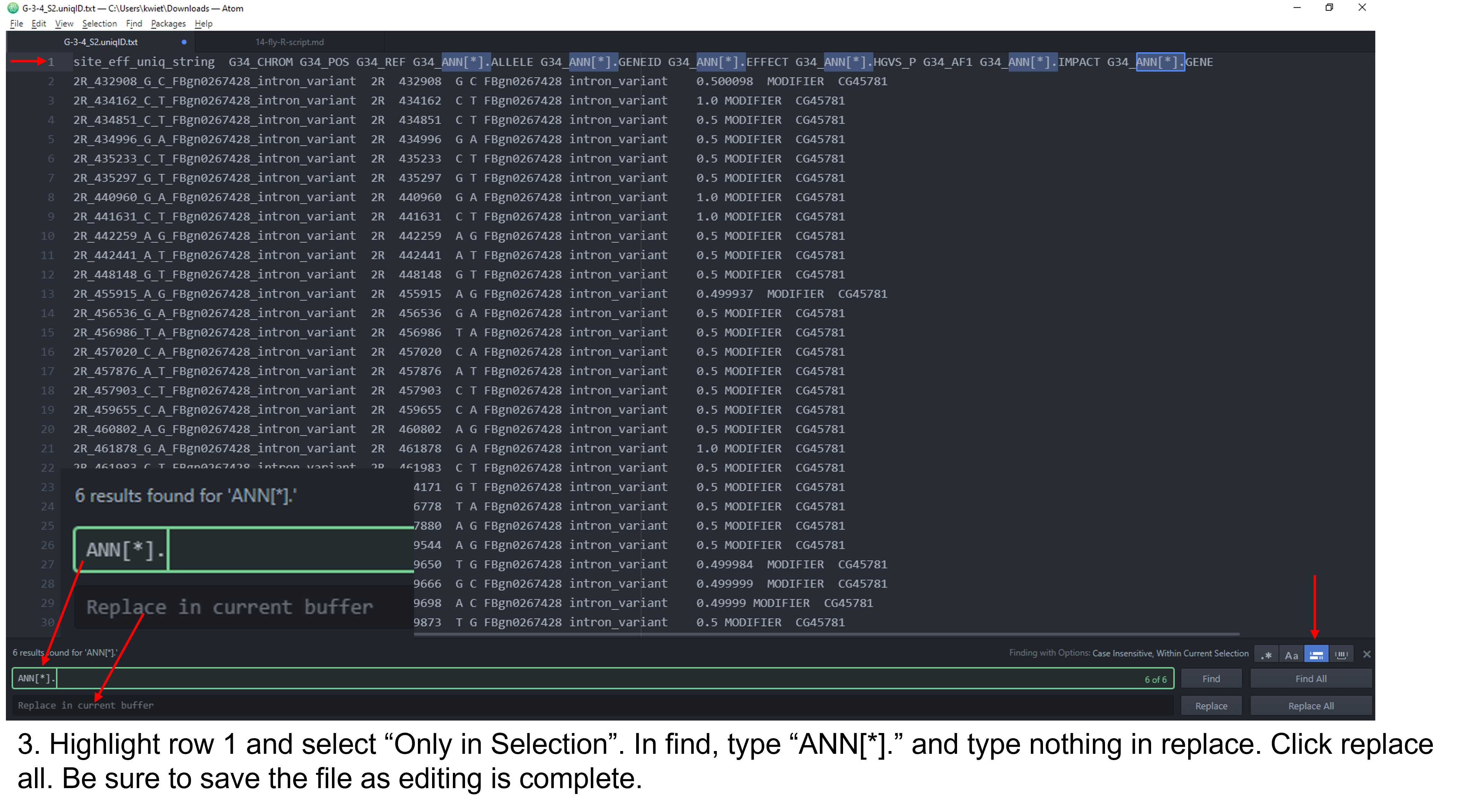
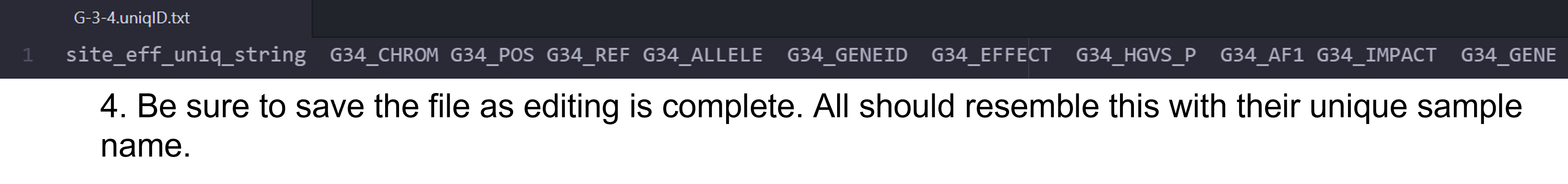Figure 2: Steps to edit column headers in Pulsar.

Open and load RStudio script

You should have already installed R and RStudio to your local machine. Additionally, you will need to download and save the snpeff_bdgp6.Rmd file located in the content library of our OneNote notebook to the same folder as your *.uniqID.txt files.

The next step is to open RStudio and create a New Project (Figure 3). Once the project is created you can open the snpeff_bdgp6.Rmd file which will load into your R project.

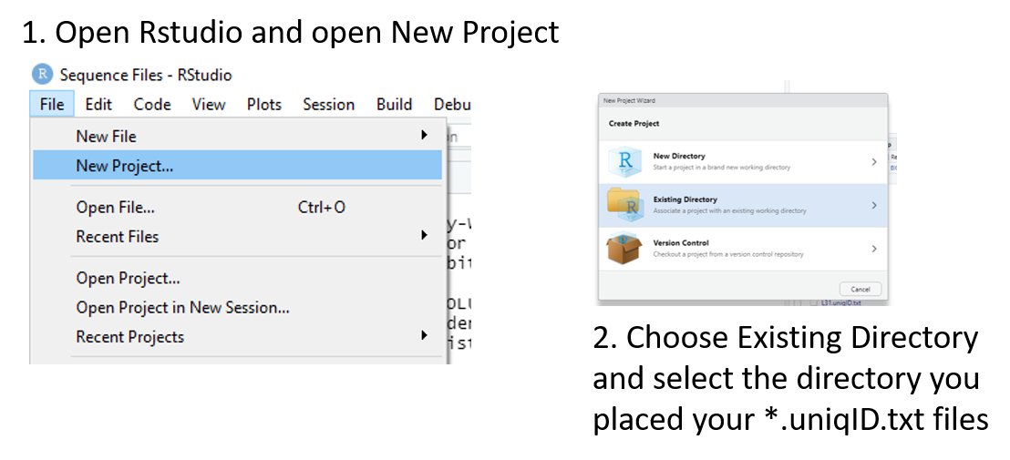Figure 3: Steps to launch a new project in RStudio.

Overview of what the R script is doing

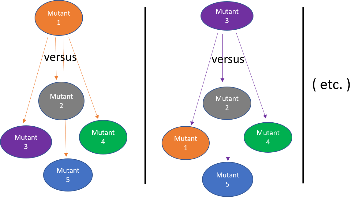Figure 4: Filtering unique Single Nucleotide Variants (SNVs) by “Round Robin” comparison.

The following script will allow you to further filter the data you obtained from the bioinformatics pipeline. Each mutant fly has accumulated numerous mutations overtime, but the majority have no effect on the phenotype (i.e. silent, non-coding, etc.). What we are interested in are mutations in protein-coding genes that appear only in a single mutant fly. The R script will compile all the mutations identified in all 5 of the flies you selected and then filter that list to generate a single file for each mutant fly that contains only mutations present in that fly and absent from the 4 other comparison flies. For example, all mutations present in mutant fly #1, will be compared to all the mutations in flies 2-5 (Fig. 4). A spreadsheet will be generated for mutant fly #1 containing only mutations present in fly #1 and absent from flies 2-5. The same “round-robin” comparison is then done for flies 2-5 resulting in 5 .tsv files (which you can view in Excel) of mutations identified that are unique to (uniq2) that single mutant.

Run the RStudio script

The purpose of this R script is to obtain a list of unique SNPs present in each of the mutant fly stocks. The input files for this script will be the text files generated from the SnpSift script that was the last step in our variant calling workflow in JupyterLab. Let’s break down what each chunk (the official term in R) of code is doing.

Chunk 1 is just the title of our notebook and it’s output format. (In R, the sections of code are called Chunks.)

---
title: "R Notebook"
output: html_notebook
---

Chunk 2 are three library’s that are loaded into R to conduct our analysis. Below is a brief description of their functions. If R states you need to install updates, please do so. -readr: The goal of ‘readr’ is to provide a fast and friendly way to read rectangular data (like ‘csv’, ‘tsv’, and ‘fwf’). -dplyr: A package which provides a set of tools for efficiently manipulating datasets in R. -tidyr: Ensures your data is tidy and states every column is a variable, every row is an observation, and every cell is a single value.

```{r mylibs}
# library loading chunk
library("readr")
library(dplyr)
library(tidyr)
```

Hit the play button (Fig. 5).

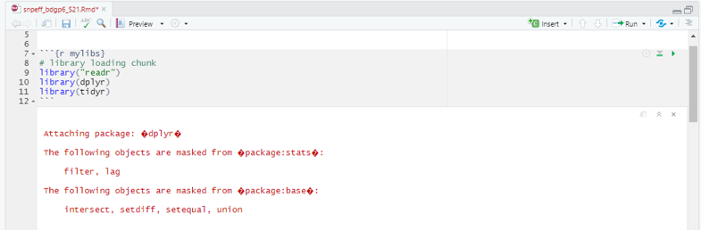Figure 5: Chunk 2 and it’s output.

Chunk 3 is our data importing chunk. R has an idea of where it is located just like our data structure in the terminal. Thus, if this R script is within the same folder as the *.uniqID.txt files, when this chunk is played, it should automatically be able to find the text files. Notice we are using ./ to indicate that the text files are “right here”. If you start to receive any errors, one possibility is that your column headers aren’t exactly as shown in the previous steps. Each of these chunks are written assuming the text headers as described in order to function.

```{r importing}
# data import chunk
frameA44<-read_tsv("./A44.uniqID.txt")
frameL32<-read_tsv("./L-3-2_S3.uniqID.txt")
frameN11<-read_tsv("./N-1-1_S4.uniqID.txt")
frameB13<-read_tsv("./B-1-3_S1.uniqID.txt")
frameO22<-read_tsv("./O-2-2_S5.uniqID.txt")
```

Hit the play button (Fig. 6).

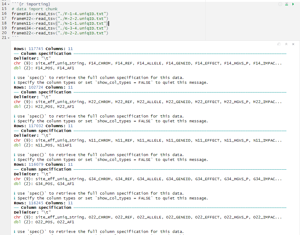Figure 6: Chunk 3 and it’s output.

Chunk 4. We have named this chunk mega join, because we are joining all of the SNPs that were generated from our previous outputs. We are doing this by using the first column of each file (site_eff_uniq_string). This will generate an all_genic_snps.tsv file that will display what reference nucleotide (Ref = genomic reference) and mutant nucleotide (Allele = mutant stock) was identified for a specific genomic location from all of the fly stocks. If there is a difference in nucleotides at a specific genomic location, the Ref and Allele columns will display different nucleotides. If no nucleotides are displayed in these columns for a specific fly stock, that means there was no difference in nucleotides between Ref and Allele at those specific locations. This will be a very large file, but you can take a peak at it within R itself. The primary purpose of this step is to organize all of the fly stocks in comparison to one another so that we can pull out only the SNPs that are unique to a single stock.

```{r mega_join}
all_snp_frames <- frameA44 %>%
  full_join(frameL32, by = "site_eff_uniq_string") %>%
  full_join(frameN11, by = "site_eff_uniq_string") %>%
  full_join(frameB13, by = "site_eff_uniq_string") %>%
  full_join(frameO22, by = "site_eff_uniq_string")
```

Hit the play button (Fig. 7).

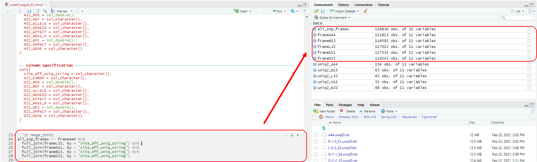Figure 7: Chunk 4 and it’s output.

Chunk 5 conducts pair-wise comparisons between the first stock listed (i.e. uniq2_A44) to each of the other 9 fly stocks. This will ultimately generate a list of SNPs that are present only in this particular stock (i.e. mutant stock A44).

```{r}
### select sets from the all_snp_frames
uniq2_A44<-all_snp_frames %>% filter(is.na(L32_POS),is.na(N11_POS),is.na(B13_POS),is.na(O22_POS),A44_EFFECT!="synonymous_variant",A44_IMPACT!="MODIFIER") %>% select(site_eff_uniq_string,starts_with("A44"))
uniq2_L32<-all_snp_frames %>% filter(is.na(A44_POS),is.na(N11_POS),is.na(B13_POS),is.na(O22_POS),L32_EFFECT!="synonymous_variant",L32_IMPACT!="MODIFIER") %>% select(site_eff_uniq_string,starts_with("L32"))
uniq2_N11<-all_snp_frames %>% filter(is.na(A44_POS),is.na(L32_POS),is.na(B13_POS),is.na(O22_POS),N11_EFFECT!="synonymous_variant",N11_IMPACT!="MODIFIER") %>% select(site_eff_uniq_string,starts_with("N11"))
uniq2_B13<-all_snp_frames %>% filter(is.na(A44_POS),is.na(L32_POS),is.na(N11_POS),is.na(O22_POS),B13_EFFECT!="synonymous_variant",B13_IMPACT!="MODIFIER") %>% select(site_eff_uniq_string,starts_with("B13"))
uniq2_O22<-all_snp_frames %>% filter(is.na(A44_POS),is.na(L32_POS),is.na(N11_POS),is.na(B13_POS),O22_EFFECT!="synonymous_variant",O22_IMPACT!="MODIFIER") %>% select(site_eff_uniq_string,starts_with("O22"))
```

Hit the play button (Fig. 8).

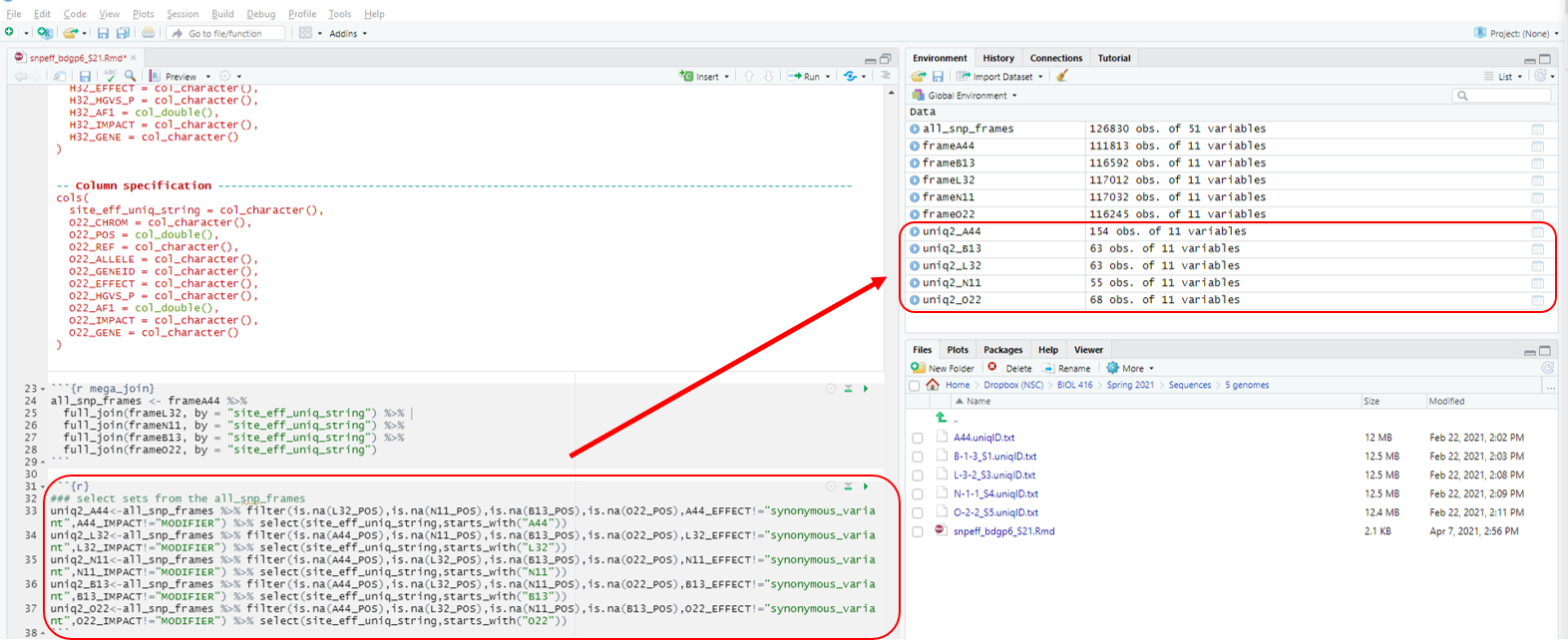Figure 8: Chunk 5 and it’s output.

Chunk 6 exports the data to a tab-delimited format that you can open in excel using the default prompts. After you hit the play button you should see new files in the folder that the original text files are in. I suggest opening excel and then opening each of the files from there. Give yourself a big pat on the back as you have just finished the bioinformatics analysis pipeline in our quest to identify the causative SNP in each of the fly mutants!

```{r}
### file export
uniq2_A44 %>% write_tsv("./prioritySNPs_A44.tsv")
uniq2_L32 %>% write_tsv("./prioritySNPs_L32.tsv")
uniq2_N11 %>% write_tsv("./prioritySNPs_N11.tsv")
uniq2_B13 %>% write_tsv("./prioritySNPs_B13.tsv")
uniq2_O22 %>% write_tsv("./prioritySNPs_O22.tsv")
all_snp_frames %>% write_tsv("./all_genic_snps_all.tsv")
```

Hit the play button (Fig. 9).

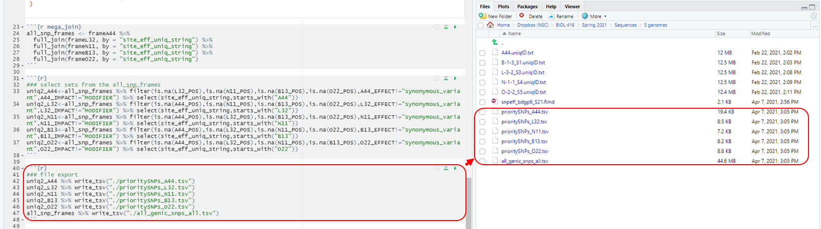Figure 9: Chunk 6 and it’s output.

But now what?!?!

You can view each of the .tsv files in Microsoft Excel. I suggest opening excel first, and then searching to open the .tsv file. You can accept any of the prompts that may show up. Your final exam will have you analyzing your data to identify a causative SNP in these mutant Drosophila melanogaster. Your final exam is available in the Class Notebook.

Key Points

• R script used to generate useable list of unique SNPs for each mutant.

• End of the bioinformatics pipeline.